Dynamic Programming: Get Started in 2 Minutes

Bellman, the mathematician who introduced dynamic programming, said, “Dynamic programming amounts to breaking down an optimization problem into simpler sub-problems, and storing the solution to each sub-problem so that each sub-problem is only solved once”.
Jonathan Paulson explains dynamic programming (DP) in his amazing Quora answer here:
Writes down "1+1+1+1+1+1+1+1 =" on a sheet of paper.
"What's that equal to?"
Counting "Eight!"
Writes down another "1+" on the left.
"What about that?"
"Nine!" " How'd you know it was nine so fast?"
"You just added one more!"
"So you didn't need to recount because you remembered there were eight!
Dynamic Programming is just a fancy way to say remembering stuff to save time later!"
Why to use it?#
There is a famous saying,
“Those who cannot remember the past are condemned to repeat it.”
Dynamic programming can be stated as,
DP = Recursion + Caching
Caching is storing every value ever calculated. This eliminates repeated recursive calls and saves a lot of time. One can invoke recursion to solve a problem by DP. But it is not necessary. One can solve DP without recursion too.
The intuition behind dynamic programming is that we trade space for time, i.e. to say that instead of calculating all the states taking a lot of time but no space, we take up space to store the results of all the sub-problems to save time later.
It can be used to solve many problems in \(O(n2)\) or \(O(n3)\) polynomial time for which a naive approach would take exponential time.
When to use it?#
A problem needs to have two key attributes in order for DP to be applicable:
- Optimal substructure: An optimal solution to a problem contains optimal solutions to subproblems
- Overlapping subproblems: When you might need the solution to the sub-problems again. A recursive solution contains a “small” number of distinct subproblems repeated many times.
Simply, the basic idea is to break a problem up into subproblems, find optimal solutions to subproblems to give us optimal solutions to the larger ones, and in the process store every value calculated to prevent repeated calculations.
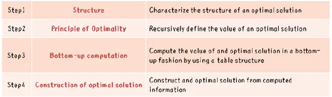
Every DP problem has four steps:
Show that the problem can be broken down into optimal sub-problems.
Recursively define the value of the solution by expressing it in terms of optimal solutions for smaller sub-problems.
Compute the value of the optimal solution in a bottom-up fashion.
Construct an optimal solution from the computed information.
It is similar to “divide-and-conquer” as a general method (mergesort, quicksort), except that unlike divide-and-conquer, the subproblems will typically overlap. Note that if a problem can be solved by combining the optimal solution of non-overlapping subproblems then we are in the “divide and conquer” area, where for example merge sort and quick sort lies.
Two dynamic programming approaches:#
- Bottom-Up (Tabulation): I’m going to learn to program. Then, I will start practicing. Then, I will start taking part in contests. Then, I’ll practice even more and try to improve. After working hard like crazy, I’ll be an amazing coder.
- Top-Down (Memoization): I will be an amazing coder. How? I will work hard like crazy. How? I’ll practice more and try to improve. How? I’ll start taking part in contests. Then? I’ll practice. How? I’m going to learn to program.
Let’s get into an example: Fibonacci sequence#
For overlapping subproblems:#
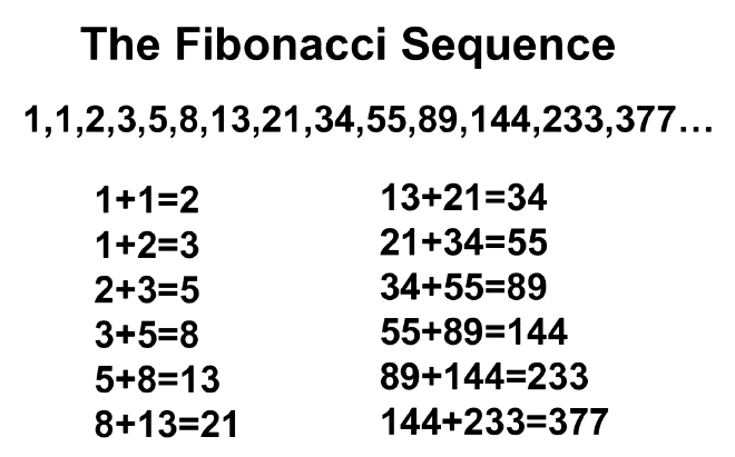
The recurrence relation for Fibonacci is \(F_n = F_{n-1} + F_{n-2}\)
The naive recursive program for fibonacci sequence takes \(O(2^n)\) :
int fibo(int n)
{
    if(n <= 1){ return n; }
    return fibo(n-1) + fibo(n-2);
}
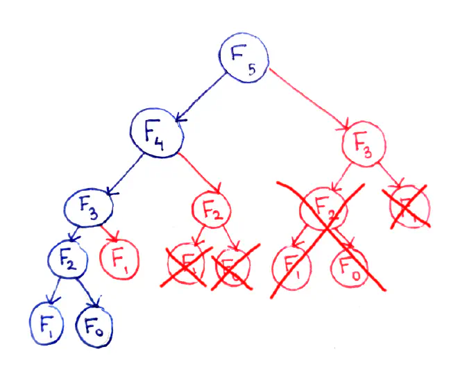
The recursion tree for the execution of fibo(5):
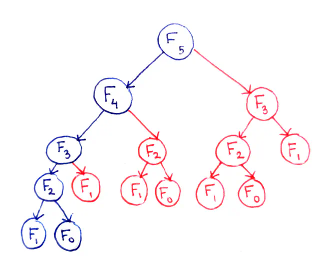
The fundamental issue here is that certain subproblems are computed multiple times. For example, F(3) is computed twice, and F(2) is computed three times (overlapping of subproblems), despite the fact they will produce the same result each time. We can save a lot of time if we cache them.
Let’s try the memoization approach (top-down)#
Starts with higher values of input and keep building the solutions for lower values.
- The memoized program for a problem is similar to the recursive version with a small modification that it looks into a lookup table before computing solutions.
- We initialize a lookup array with all initial values as NIL.
- Whenever we need solution to a subproblem, we first look into the lookup table.
- If the precomputed value is there then we return that value, otherwise we calculate the value and put the result in lookup table so that it can be reused later.
#include<bits/stdc++.h>
using namespace std;
#define NIL -1
#define MAX 1000

long long lookup[MAX];

void fill()
{
	memset(lookup, NIL, MAX * sizeof(lookup[0]));
}
long long fibo(int n)
{
	if(lookup[n] == NIL)
	{
		if(n <= 1)
			lookup[n] = n;
		else
			lookup[n] = fibo(n - 1) + fibo(n - 2);
    }
    return lookup[n];
}
int main()
{
	int n;
	cout<<"Enter n: ";
	cin>>n;
	fill();
	cout<<"Fibonacci number is "<<fibo(n);
	return 0;
}
By caching the results of subproblems, many recursive calls are eliminated. The time complexity has been reduce to O(n) and the space complexity is also same.
Let’s try the tabulation approach (bottom up)#
Starts with lower values of input and keep building the solutions for higher values.
- The tabulated program for a given problem builds a table in bottom up fashion and returns the last entry from table
- So for the same Fibonacci number, we first calculate fib(0) then fib(1) then fib(2) then fib(3) and so on.
- Literally, we are building the solutions of subproblems bottom-up.
#include<bits/stdc++.h>
using namespace std;

long long fibo(int n)
{
	long long f[n+1];
	f[0] = 0; f[1] = 1;
	for(int i=2;i<=n;i++){
	    f[i] = f[i-2] + f[i-1];
	}
	return f[n];
}
int main()
{
	int n;
	cout<<"Enter n: ";
	cin>>n;
	cout<<"Fibonacci number is "<<fibo(n);
	return 0;
}
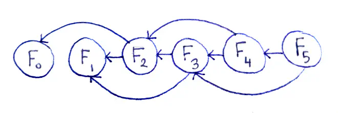
Drawing out each subproblem only once makes the relations between the subproblems clearer.
This representation is useful for a number of reasons. First, we see that there are O(n) subproblems. Second, we can see the diagram is a directed acyclic graph (or DAG for short), meaning:
- There are vertices (the subproblems) and edges between the subproblems (dependencies).
- The edges have a direction, since it matters which subproblem for every connected pair is the dependent one.
Both the time and space complexity is \(O(n)\). The iterative approach is the most efficient way to find Fibonacci numbers since it reduces space complexity to \(O(1)\) in \(O(n)\) time. Since it has nothing to do with DP, I won’t discuss it here.
Note that for all problems, it may not be possible to find both top-down and bottom-up solutions.
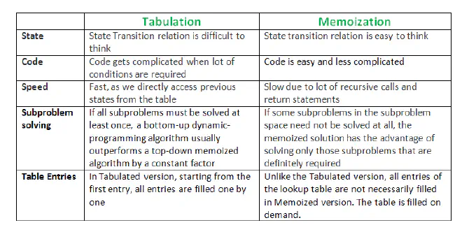
Both the approaches stored the solutions of subproblems. In Memoized version, the table is filled on demand while in the Tabulated version, starting from the first entry, all entries are filled one by one. Unlike the Tabulated version, all entries of the lookup table are not necessarily filled in the Memoized version.
Another example: Bellman-Ford algorithm for finding shortest path#
For optimal substructure:#
- A given problem has the optimal substructure property if the optimal solution of the given problem can be obtained by using the optimal solutions of its subproblems.
- For example, the Shortest Path problem has following optimal substructure property: “If a node x lies in the shortest path from a source node u to destination node v then the shortest path from u to v is a combination of the shortest path from u to x and shortest path from x to v”
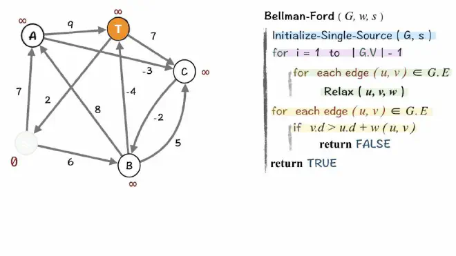
- What do we use here? Bellman-ford algorithm for finding the shortest path.
- Given a graph and a source vertex src in the graph, find the shortest paths from src to all vertices in the given graph. The graph may contain negative weight edges.
We need a bottom-up approach!#
- First, calculate the shortest distances which have at-most one edge in the path.
- Then, calculate the shortest paths with at-most 2 edges, and so on.
- After the ith iteration of the outer loop, the shortest paths with at most i edges are calculated.
- There can be maximum \(|V| – 1\) edges in any simple path, that is why the outer loop runs \(|v| – 1\) times.
- The idea is, assuming that there is no negative weight cycle if we have calculated the shortest paths with at most i edges, then an iteration over all edges guarantees to give the shortest path with at-most \((i+1)\) edges
References:
- https://youtu.be/DiAtV7SneRE
- https://github.com/llSourcell/dynamic_programming/blob/master/Dynamic%20Programming.ipynb
- https://medium.com/future-vision/a-graphical-introduction-to-dynamic-programming-2e981fa7ca2
- http://blog.gaurav.im/2017/08/16/dynamic-programming-you-can-do-it-half-asleep/
- https://www.hackerearth.com/practice/algorithms/dynamic-programming/introduction-to-dynamic-programming-1/tutorial/